|
RayZaler 0.1
The free opto-mechanical simulation framework
|
|
RayZaler 0.1
The free opto-mechanical simulation framework
|
Existing optical simulation software usually relies on some sort of integrated model editor that acts as the only interface between the user and the model itself. While this is enough in most cases, in some others it is not. A typical scenario is the following: there are multiple people working on the same model, each one modifying different parts of it. How do we put all these changes together? How do we keep track of the changes across versions? Another difficulty arises when we get back to a model we have bot been working on in a while. Why are certain elements arranged the way they are? And finally, why should the user install a full-fledged simulation suite just to get a glimpse of how a model is made?
These difficulties were part of the motivation behind RayZaler, and the way we addressed it was simple: plain text model files. RayZaler models are created pretty much as you would create any script file: pick your favourity text editor, specify which elements there are in your model and how they are arranged, verify it with RZGUI and that is it. That is how you create model files.
Model files are written in the so-called RayZaler Modelling Language, and usually bear the extension .rzm (although it is not mandatory). Model files can also incorporate definitions from other files via inclusion, letting you define libraries of complex optical systems. These include files usually bear the extension .rzi although, once again, this is merely a suggestion.
The best way to learn how to write model files is by example. Consider a simple newtonian telescope (parabolic primary mirror + flat secondary mirror) with the following specifications:
We can do the math and deduce the plate scale of this telescope:
$$ p\approx \frac{206265 \text{"/rad}}{1200\text{ mm}}\approx 172\text{"/mm} $$
Meaning that each pixel in the detector corresponds to an angle in the sky of roughly 2.6 arcsec.
Let us start by modelling the primary mirror. Open your favourite text editor and create a file with the following contents:
ParabolicMirror M1;
This is the most basic definition of an element in a model. It consists of a parabolic mirror (ParabolicMirror) we arbitrarily named M1. RayZaler supports an (ever growing) variety of optical and non-optical elements, and ParabolicMirror is one of them. Parabolic mirrors are a particular case of a more general element class, the conic mirror (ConicMirror) which enables the definition of mirrors with curved surfaces parametrized by their curvature radius and conic constant.
If you have a superficial knwoledge of languages like C++ or Java, the contents of the file may feel familiar to you. In particular, it looks like the instantiation of an object named M1 from the class ParabolicMirror. This is intentional: internally, RayZaler will create an instance of the class ParabolicMirror, which can be later queried and accessed from the C++ / Python APIs.
Save this file as telescope.rzm and visualize its contents by mean of RZGUI. You can do this in two ways:
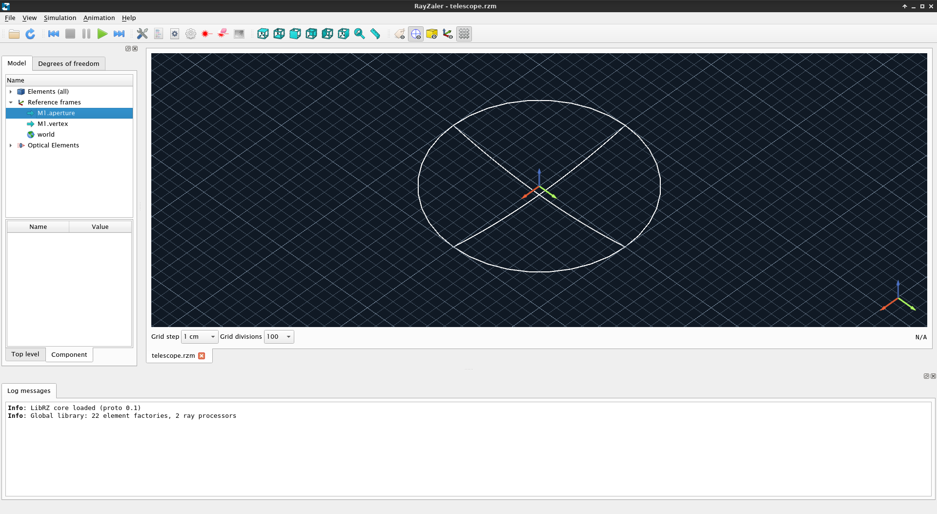
telescope.rzm and run RZGUI telescope.rzm, orRZGUI as-is, either from the terminal or the "run command" window of your favourite desktop environment and open telescope.rzm from the File → Open menu.In either case, you should see something like this:
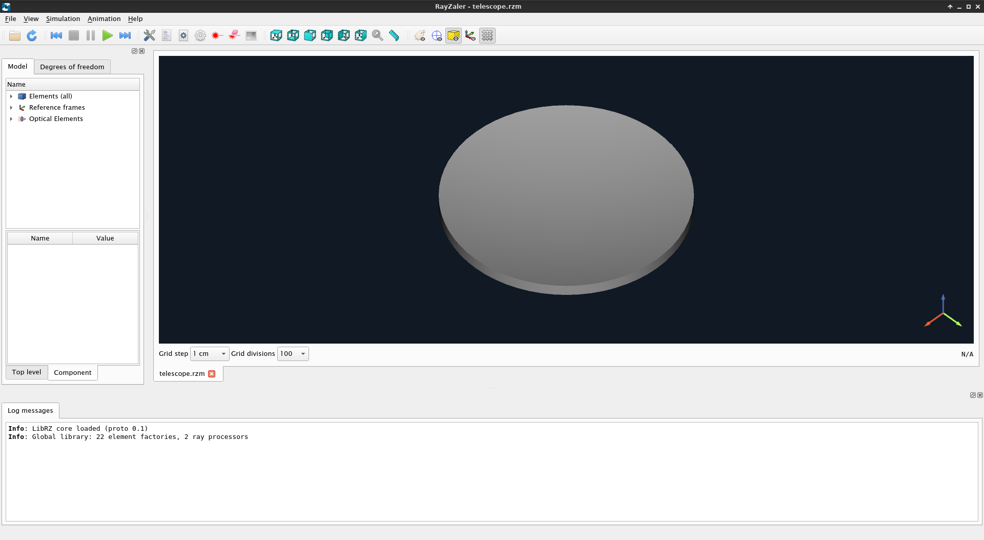
This is our primary mirror, as displayed by RZGUI. This is an interactive representation of the model you can navigate with your keyboard and mouse:
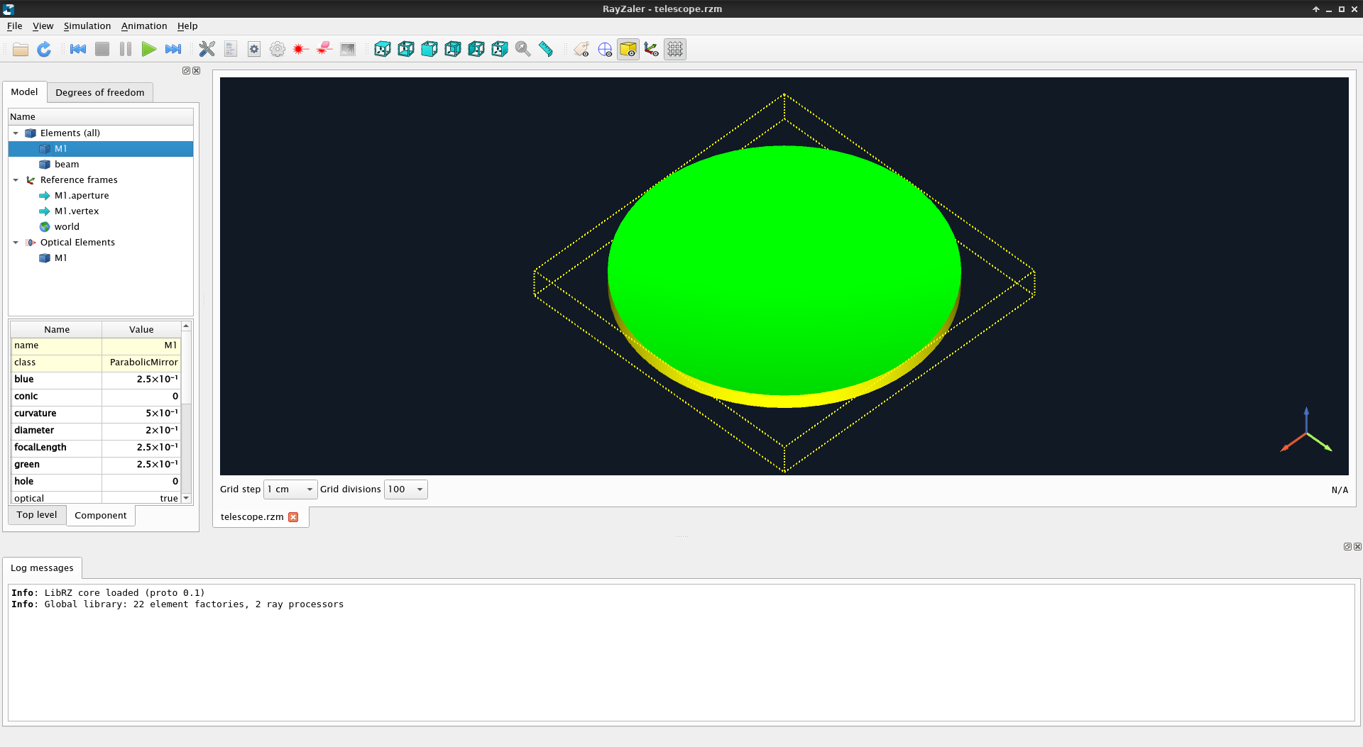
RZGUI can be used to inspect additional features of the model. If you click on Elements it will unfold into two items: M1 and beam. The former is the parabolic mirror we defined earlier. The latter is used to represent the rays of the latest simulation and exists in all models. However, since we have not run any simulation yet, it is effectively invisible.
Click now on M1. This highlights both the element and its bounding box. Some elements (like mirrors or lenses) have an orientation, with a front side and a back side. The front side is always highlighted in green and the back side in red. All other faces are highlighted in yellow.
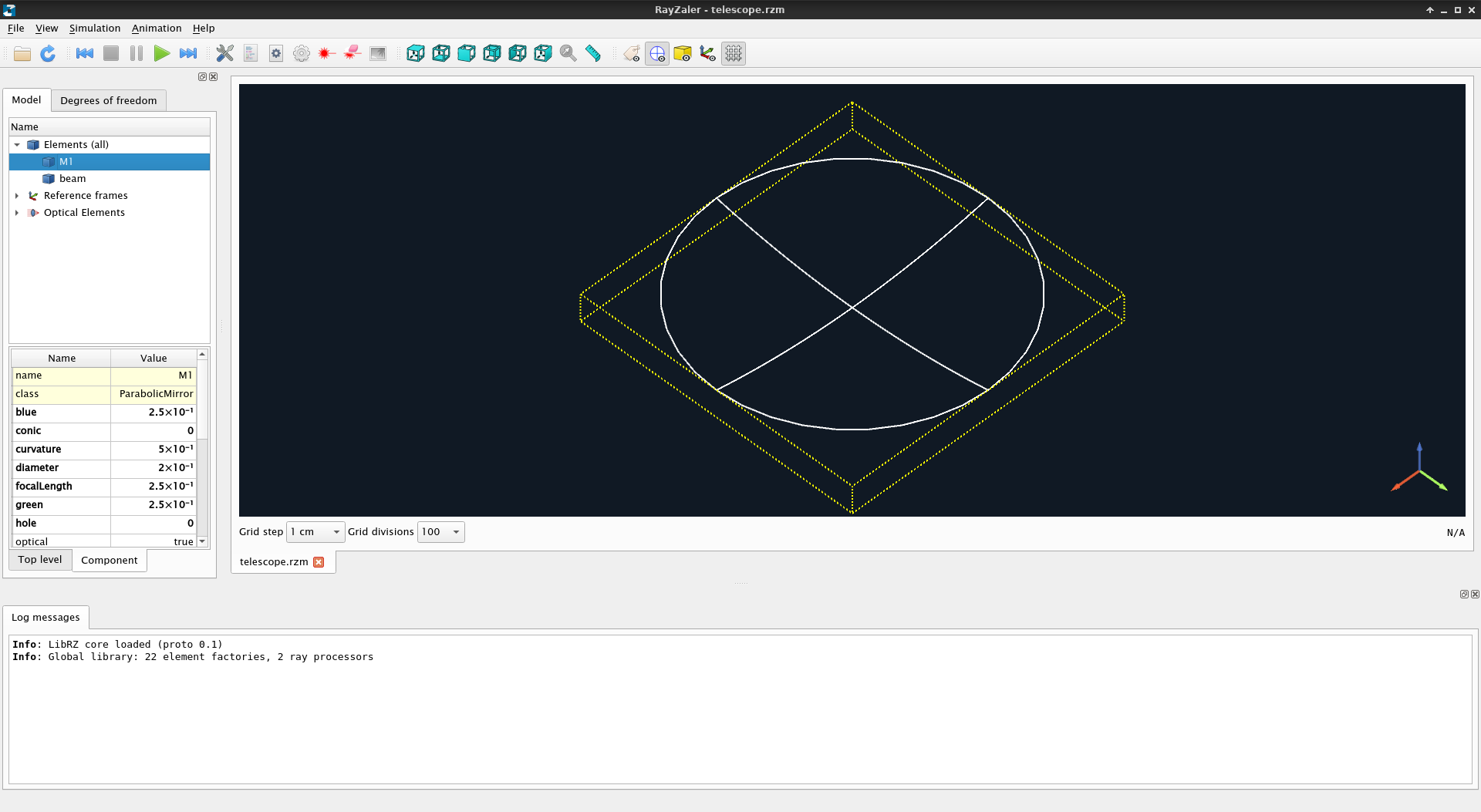
An optical element is just an element in the model that interacts with light, and may consist of one or more optical surfaces. These surfaces may be the surface of a mirror, or an interface between two media.
You can highlight the optical surfaces of a model by clicking on Toggle display optical surfaces. By clicking on Toggle display elements you can hide the 3D representation of elements and show their surfaces alone.

Now click on Reference frames. This entry will unfold in the following items:
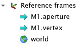
Reference frames are the primitives provided by RayZaler to position elements in a model. They represent a coordinate center and an orientation of the axes. All elements in a model are specified with respect to a given reference frame.
When no reference frame is specified, an element is placed inside the world reference frame. It represents certain global reference frame with respect to which all other reference frames are defined.
Additional reference frames can be created either explicitly by the user (we will see more of this later on) or by other elements. For instance, in this case, the mirror M1 exposes two additional reference frames: aperture (centered in the plane containing the circular edge of the mirror) and vertex (centered in the plane tangent to the parabolic surface of the mirror in its center.
Click on M1.aperture and M1.vertex. This action will display a grid and 3 coloured axes, representing the center and orientation of the corresponding reference frame. The red arrow is aligned with the X axis, the green arrow with the Y axis and the blue arrow with the Z axis. Generally, reference frames depending on optical surfaces tend to align the Z axis with the surface normal at the center (vertex).
If no further information is provided, the parabolic mirror is created with some arbitrary defaults. In this case, 20 cm in diameter, 25 cm focal length and 1 cm thickness. However, the original specification required a 254 mm telescope with 1200 mm focal length. We can adjust these properties by specifying them in the primary mirror definition:
ParabolicMirror M1(focalLength = 1200e-3, diameter = 254e-3);
This line defines a parabolic mirror with parameters focalLength set to 1200e-3 and diameter set to 254e-3. These are the properties used in parabolic mirrors to define the focal length and diameter respectively, although we could also have used the curvature radius instead (property curvature) or the radius of the mirror (property radius).
Note the e-3 suffix with no spaces. This is read as \((...)\times10^{-3}\), implying that both the focal length and the diameter are are expected to be given in meters. In RayZaler, all length quantities are always specified in meters, and angular quantities in degrees. We could also have written the line above as:
ParabolicMirror M1(focalLength = 1.2, diameter = 0.254);
Save the file and, in RZGUI press the keyword combination Ctrl + R to reload the model with the new changes. You should see now that the M1 has increased its size.
Below the Model tab you should see a table with two columns, Name and Value. This table summarizes the properties of the selected component. Click on M1 in the Model tab and, in the property table, kicate focalLength and diameter. The values should be $1.2$ and $2.54\times10^{-1}$ respectively, meaning that the properties were adjusted accordingly.
RayZaler provides three different positioning primitives: translate, rotate and on...of. All of them are used to define the reference frame with respect to which the following statement(s) is(are) processed. They have a syntax of the form:
<primitive> {
  # Element definitions go here
}
meaning that everything enclosed by the curly braces is defined with respect to that reference frame. They can arbitrarily nested:
<primitive1> {
  # Element definitions inside primitive1
  <primitive2> {
    # Element definitions inside primitive2 (defined respect primitive1)
  }
  # Element definitions inside primitive1 again
}
For instance, the following code:
translate(dy = 100e-3) {
  rotate(30, 1, 0, 0) {
    ConicLens L1;
  }
}
Creates a lens that is rotated 30º around the X axis ($\mathbf k=(1, 0, 0)^\top$), 100 mm away in the Y direction with respect to the current frame.
Positioning primitives are generally non-commutative. The previous code is not equivalent to the following:
rotate(30, 1, 0, 0) {
  translate(dy = 100e-3) {
    ConicLens L1;
  }
}
Which would rotate the system around the X axis first (meaning that both the Y and Z axes now point to different directions), and then displace the reference frame in the rotated Y direction.
Finally, if there is only one statement inside the positioning primitive, we can get rid of the curly braces altogether:
translate(dy = 100e-3)
  rotate(30, 1, 0, 0)
    ConicLens L1;
Note that model files treat spaces, tab spaces and line breaks the same way. What actually marks the end of a statement is the semicolon (;). This means that one-liners like this are also accepted:
translate(dy = 100e-3) rotate(30, 1, 0, 0) ConicLens L1;
The translate primitive is used to create a new reference frame that is translated with respect to the current reference frame, keeping the same orientation. The syntax is as follows:
translate(dx = <DX>, dy = <DY>, dz = <DZ>) {
  ...
}
where <DX>, <DY> and <DZ> are the displacements in the X, Y and Z axes respectively, in meters. All displacements are optional, and when they are not specified they default to 0. For instance:
translate(dx = 3e-2) {
  translate(dy = -2e-2) {
    ...
  }
}
is equivalent to:
translate(dx = 3e-2, dy = -2e-2) {
  ...
}
The rotate primitive is used to create a new reference frame that is rotated with respect to the current reference frame, keeping the same center. Rotations in RayZaler are specified by means of the axis-angle representation. The syntax of this primitive is:
rotate(<ANGLE>, <Ux>, <Uy>, <Uz>) {
  ...
}
where <ANGLE> is the right-handed rotation angle in degrees, and <Ux>, <Uy>, <Uz> are the components of the rotation axis vector, normalized or not. For instance, a rotation of 90º around the Y axis is specified as:
rotate(90, 0, 1, 0) { ... }
Some elements define useful reference frames that can be used as origin of the definition of additional elements or reference frames. For instance, BlockElement elements are non-optical elements representing a rectangular prism with a width, height and length, and exposing 6 reference frames (top, bottom, left, right, front, back) located in each side of the prism. The on ... of primitive is used to enter in these element-relative reference frames.
Unlike the rotate and translate primitives (which are relative to the current reference frame, and therefore are sensitive to the order in which they are applied), on ... of can appear anywhere and be applied in any order, as they represent certain absolute jump into a new reference frame.
The syntax of the on ... of primitive is as follows:
on <FRAME> of <ELEMENT> {
  ...
}
where <FRAME> is the named reference frame of the previously defined element <ELEMENT>. For instance:
BlockElement box;

on top of box {
  FlatMirror M1;
}
will create a flat mirror named M1, placed on top of the element named box.
The secondary mirror of a Newtonian telescope is a simple flat mirror located somewhere along the optical axis of the telescope with a 45º tilt towards the eyepiece / detector. RayZaler provides an optical element for this type of mirrors (FlatMirror) which can be defined either by their radius, their diameter, or their width and height. However, according to the system prescription, this mirror is located 600 mm ahead the center (vertex) of the mirror. In other words, we have to define additional reference frames.
The sequence of reference frame changes we need to do before placing the secondary mirror is the following:
vertex frame of M1.M1's vertex in the positive Z direction.Since the last two steps are both rotations around the X axis we could merge them as a single 225º rotation and it would work. However, for better readability, we would keep these rotations separate.
Assuming we call this secondary mirror M2, we would need to update telescope.rzm as follows:
ParabolicMirror M1(focalLength = 1200e-3, diameter = 254e-3);

on vertex of M1 {
  translate(dz = 900e-3) {
    rotate(180, 1, 0, 0) rotate(45, 1, 0, 0) {
      FlatMirror M2(diameter = 110e-3, vertexRelative = true);
    }
  }
}
In the definition of the M2 we passed an additional property (vertexRelative) set to true. In RayZaler, all mirrors have a thickness, and their reflective surfaces are elevated (i.e. positively displaced in the Z axis) with respect to their parent reference frame. While this may make sense mechanically (mirrors are 3D objects), optically not so much: We would need to set the mirror thickness to a known value and translate the mirror back in the opposite Z direction by the same amount. Possible, but not too practical.
We can simplify things by setting vertexRelative = true. This way we force the center of the mirror surface to be at the center of the reference frame where it was defined, disregarding completely the actual thickness of the mirror.
We would like to do some simulations regarding the actual geometry of a detector. RayZaler provides a detector element (Detector) which mimics a CCD with a given number of rows and columns of pixels (properties cols and rows), and a pixel size (properties pixelWidth and pixelHeight). In order to match the specification, the detector must be defined as follows:
Detector det(cols = 1024, rows = 1024, pixelWidth = 15e-6, pixelHeight = 15e-6);
which ensures the detector has a resolution of 1024×1024 with 15 µm pixels.
Another requirement is to place the detector in the focal plane. But, where is the focal plane? Given that the telescope's focal length is 1200 mm and that the fold mirror is 900 mm from the ertex of the primary, we are still 1200 - 900 = 300 mm away from the focal plane. We would need an additional 45º rotation after the M2 to be aligned with the exit beam and, relative to that, move 300 mm upwards (positive Z). The updated model would look like this:
ParabolicMirror M1(focalLength = 1200e-3, diameter = 254e-3);

on vertex of M1 {
  translate(dz = 900e-3) {
    rotate(180, 1, 0, 0) rotate(45, 1, 0, 0) {
      FlatMirror M2(diameter = 110e-3, vertexRelative = true);

      rotate(45, 1, 0, 0)
        translate (dz = 300e-3)
          Detector det(
            rows = 1024,
            cols = 1024,
            pixelWidth  = 15e-6,
            pixelHeight = 15e-6);
    }
  }
}
Finally, we need to define the default optical path. This is, the ordered sequence of elements that should be traversed by light in the nominal operation of the telescope. This is required by the simulator, to know which surfaces should intercept light in each step, and which elements may introduce vignetting along the way.
Optical paths are defined by means of the path keyword, followed by the names of the optical elements in the path separated by the keyword to. In our case, light should go from M1 to M2 and from M2 to det:
ParabolicMirror M1(focalLength = 1200e-3, diameter = 254e-3);

on vertex of M1 {
  translate(dz = 900e-3) {
    rotate(180, 1, 0, 0) rotate(45, 1, 0, 0) {
      FlatMirror M2(diameter = 110e-3, vertexRelative = true);

      rotate(45, 1, 0, 0)
        translate (dz = 300e-3)
          Detector det(
            rows = 1024,
            cols = 1024,
            pixelWidth  = 15e-6,
            pixelHeight = 15e-6);
    }
  }
}

path M1 to M2 to det;
The current iteration of the model can be simulated right away. However, there is something slightly inconvenient about it: there are too many hard-coded parameters! In some cases these parameters are self-evident (like the focal length of the primary). But in some others they do not: the 300 mm displacement in the Z direction before the definition of the detector is tied to the focal length of the telescope, and if we were to change the focal length we should change this value too.
If we want to keep things consistent and reduce the number of hard-coded values, we can introduce parameters. Parameters are defined by means of the parameter keyword and behave pretty much like constants in programming languages: it is a value with a name that can be used in the definition of properties of elements and reference frames.
In general, it is a good practice to translate parameters in a specification to parameters in a model file. Additionally, comments after certain non-trivial statements are also a good idea, especially when you want to share the model with other people. Comments are prefixed by # and end with a new line.
By following these principles, a more maintainable version of the model would look like this:
parameter focalLength = 1200e-3; # Focal length of the telescope [m]
parameter M2Position  = 900e-3;  # Location of the secondary mirror [m]
parameter M1Diam      = 254e-3;  # Diameter of the primary mirror [m]
parameter M2Diam      = 110e-3;  # Diameter of the secondaty mirror [m]
parameter CCDRows     = 1024;    # Vertical resolution of the CCD
parameter CCDCols     = 1024;    # Horizontal resolution of the CCD
parameter CCDPixSize  = 15e-6;   # Side of a pixel [m]

ParabolicMirror M1(focalLength = focalLength, diameter = M1Diam);

on vertex of M1 {
  translate(dz = M2Position) {
    rotate(180, 1, 0, 0) rotate(45, 1, 0, 0) {
      FlatMirror M2(diameter = M2Diam, vertexRelative = true);

      rotate(45, 1, 0, 0)
        translate(dz = focalLength - M2Position)
          Detector det(
            rows = CCDRows,
            cols = CCDCols,
            pixelWidth  = CCDPixSize,
            pixelHeight = CCDPixSize);
    }
  }
}

path M1 to M2 to det;
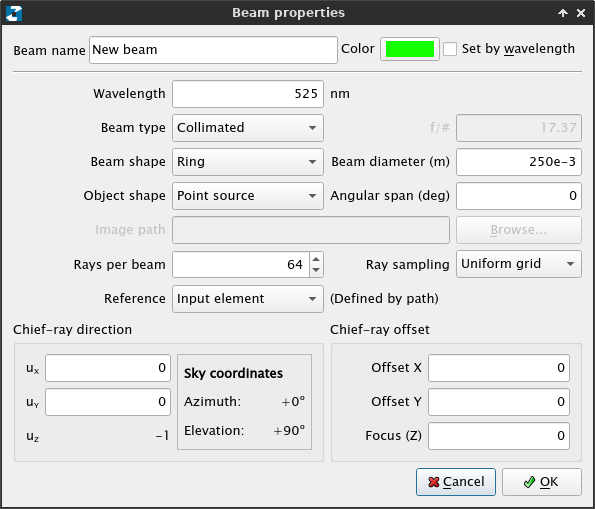
Now we are ready to test the model via simulation. In RZGUI's menu, go to Simulation → Properties to open the simulation properties dialog.
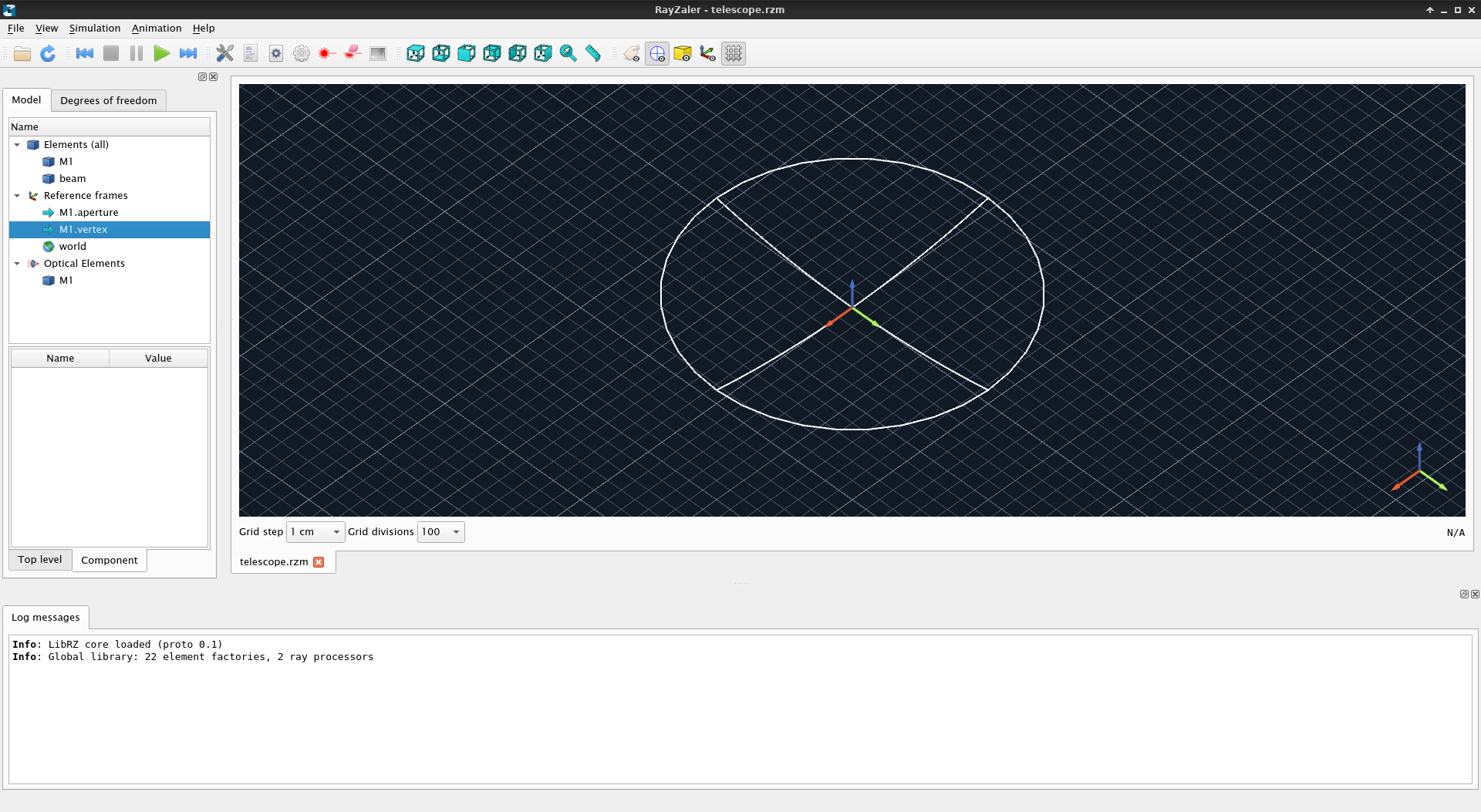
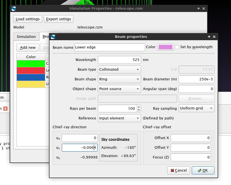
In the Beam tab, click on Add new. In the dialog that shows up, fill the blanks as follows and click OK.
Now, the Beam thab should look like this:
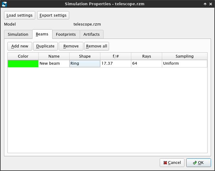
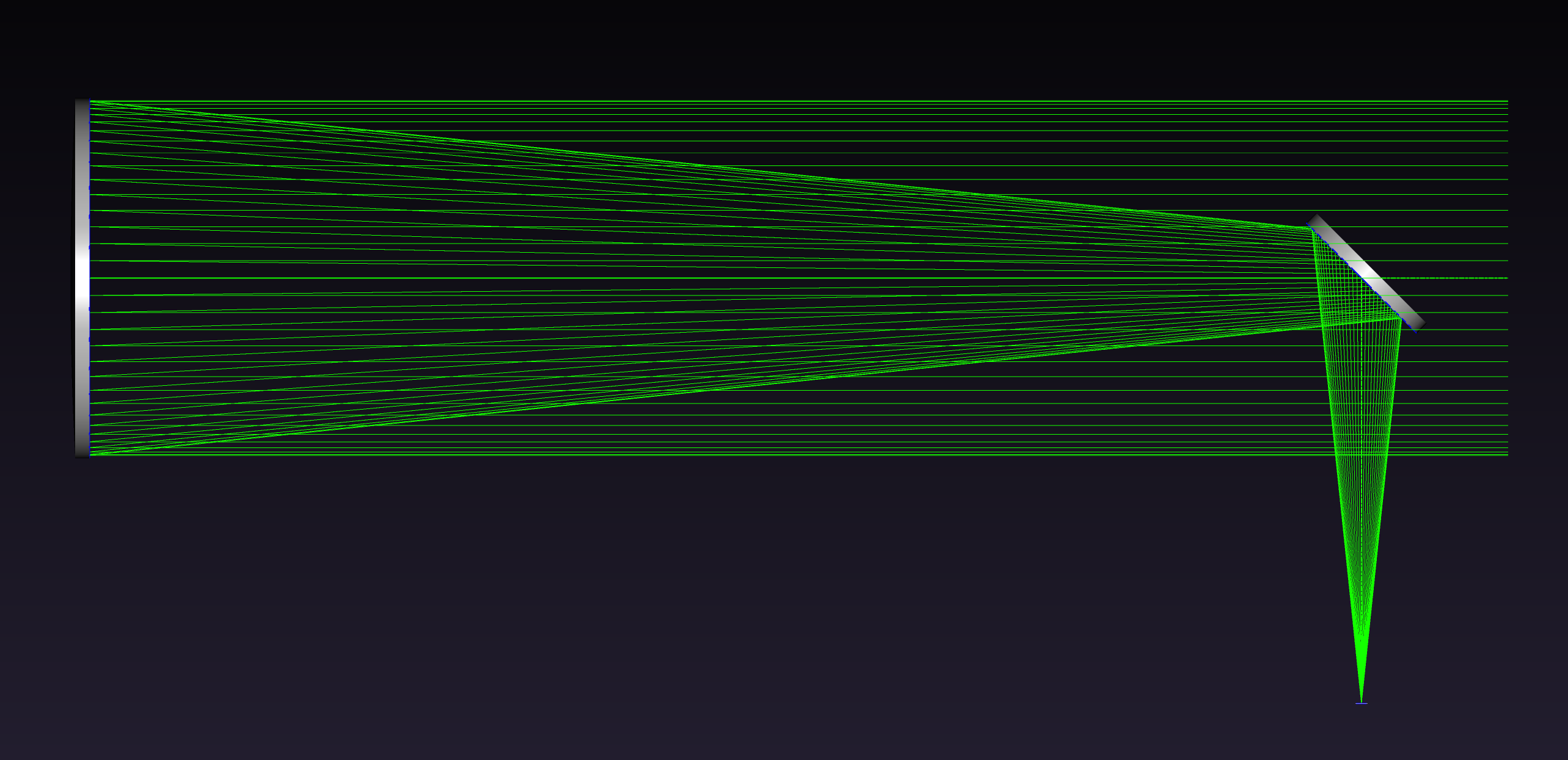
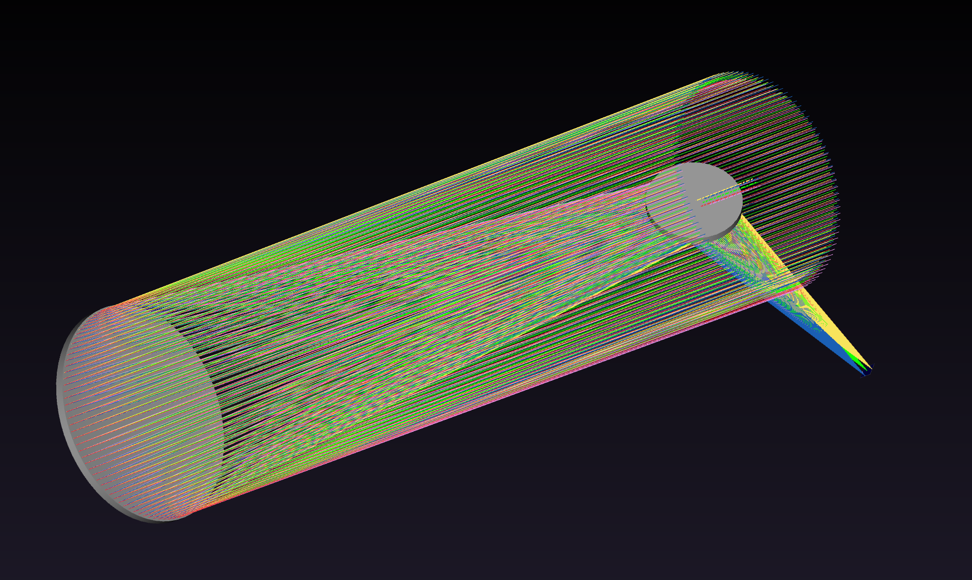
We have just defined a collimated beam with 250 mm diameter (slightly smaller than the aperture) and a ring shape, meaning that rays are only casted in the edges of the beam. Click OK again and go to Simulation→Run (or just press F5). You should see how the light enters the telescope, gets redirected by the secondary and hits the detector:
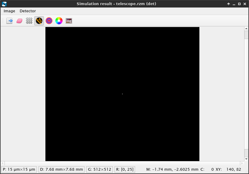
You can also inspect which pixels were illuminated by this light beam by going to Simulation→Detector window:
If you look at M2 in the simulation, you will see that the mirror is remarkably under-illuminated: the footprint is a decentered ellipse smaller than the mirror.

When this occurs, we face a suboptimal situation, not because most of the secondary is under-illumitated but because it will block more light than necessary.
We can improve the performance of the telescope by replacing the secondary mirror by an elliptical mirror. FlatMirror provides two adjustable properties for this purpose: width and height, used to set the dimensions of the mirror in the X and Y axes respectively. Setting width and height to the same value is therefore equivalent to just setting diameter.
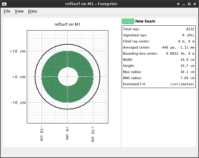
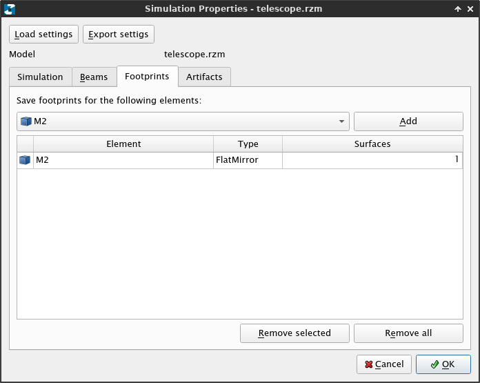
To determine appropriate center and dimensions of the secondary, we need enable the recording of beam footprints in the M2. To do this, go to Simulation → Properties, click the Footprints tab. From the drop-down list, select M2 and click Add. Click OK and repeat the simulation (F5).
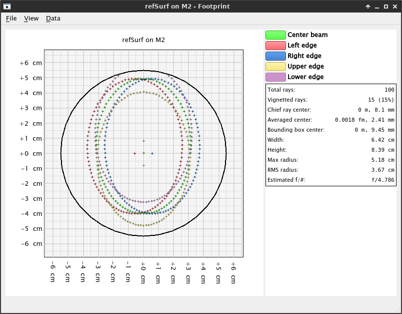
Although nothing seems to have changed, now go to Simulation → Footprints... → M2 → refSurf. This will open the footprint dialog, detailing the location of the rays hitting the reflective surface (refSurf) of the mirror M2. Click the name of the beam on the right (New beam) to see additional statistics about it:
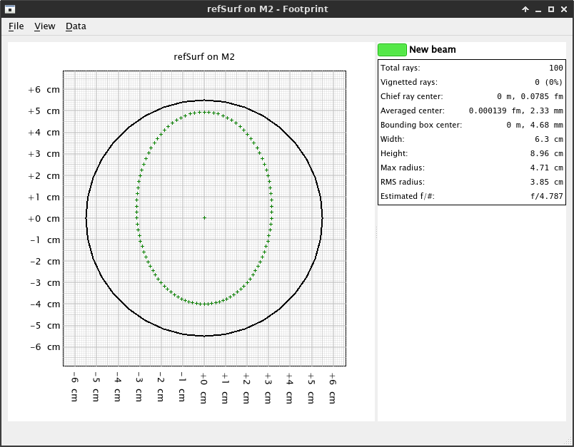
From this window we can see that, while the chief ray is almost perfectly centered, the center of the footprint shape (bounding box center) is 4.68 mm upwards. Additionally, the beam is an ellipse of 6.3 cm × 8.96 cm for a star that is perfectly aligned with the optical axis. If we observe a star that is off axis, the footprint in the M2 will also change in location and shape.
To prevent vignetting of the focused beam, we need to increase its size to make room for these off-axis starts. We can do this by casting beams to the edges of the CCD and inspecting the resulting footprints in the secondary mirror. Each of these additional beams will have direction cosines of the form $(\pm u_x, 0)^\top$ and $(0, \pm u_y)^\top$, corresponding to the projections of the edges of the CCD in the sky.
To calculate these direction cosines we proceed as follows: given that the CCD is 1024×1024 in size with 15 µm pixels, and that the focal length is 1200 mm, the edges of the CCD will be at ±7.68 mm in both directions around its center. Assuming the paraxial approximation, this translates to sky coordinates as:
$$ \Delta\theta \approx \frac{7.68}{1200} = 6.4\times10^{-3}\text{ rad } (0.367º) $$
Which can be used to approximate the direction cosines too. We need to go to Simulation &rightarrow Properties and, in the Beam tam, add new beams whose direction cosines are (-0.0064, 0), (+0.0064, 0), (0, 0.0064) and (-0, 0.0064). It is a good idea now to give different names and colors to these new beams to identify them later in the footprint dialog.
Click OK and re-run the simulation. If the simulation properties were correct, you should see something like this:
And, by zooming in the detector, you should see how the beams focus right on the edges of the detector:
Now open the footprint dialog for the M2 (Simulation → Footprints... → M2 → refSurf). We discover something interesting: not only the M2 is bigger than necessary, it introduces vignetting near the lower edge!
Fortunately, we have enough information already to fix this terrible design. By inspecting the locations of the chief rays of each beam, we observe that the max horizontal offset of the beam is of 5.77 mm both left and right, and that the max vertical offset of the beam is 8.21mm downwards. A cautions estimate of the required gap size could be 7 mm horizontally and 1 cm vertically.
From these figures, we can propose an elliptical secondary with an extra gap of 5 mm around the footprint to account for off-axis stars. This would result in a 7.7 cm × 11 cm mirror centered at 0, 4.68 mm. The updated model would look like this:
parameter focalLength = 1200e-3; # Focal length of the telescope [m]
parameter M2Position  = 900e-3;  # Location of the secondary mirror [m]
parameter M1Diam      = 254e-3;  # Diameter of the primary mirror [m]
parameter CCDRows     = 1024;    # Vertical resolution of the CCD
parameter CCDCols     = 1024;    # Horizontal resolution of the CCD
parameter CCDPixSize  = 15e-6;   # Side of a pixel [m]

parameter M2Width     = 7.7e-2;  # Width of the secondary mirror [m]
parameter M2Height    = 11e-2;   # Height of the secondary mirror [m]
parameter M2YOffset   = 4.68e-3; # Vertical offset of the secondary mirror [m]

ParabolicMirror M1(focalLength = focalLength, diameter = M1Diam);

on vertex of M1 {
  translate(dz = M2Position) {
    rotate(180, 1, 0, 0) rotate(45, 1, 0, 0) {
      translate(dy = M2YOffset)
        FlatMirror M2(width = M2Width, height = M2Height, vertexRelative = true);

      rotate(45, 1, 0, 0)
        translate(dz = focalLength - M2Position)
          Detector det(
            rows = CCDRows,
            cols = CCDCols,
            pixelWidth  = CCDPixSize,
            pixelHeight = CCDPixSize);
    }
  }
}

path M1 to M2 to det;
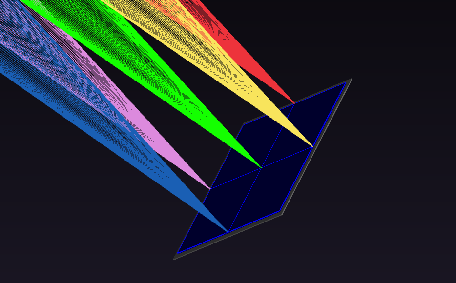
And, if we repeat the simulation, now the footprint of the beams at the M2 will look like this:
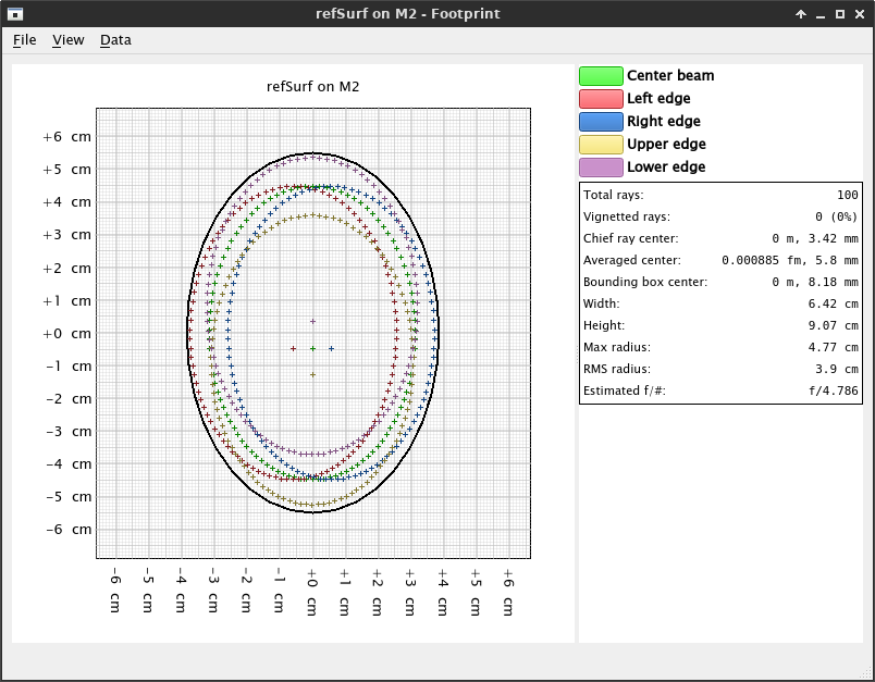
A much tighter fit than the previous M2, and with no vignetting!
We have a model that looks like what we would ask for an ideal telescope. However, real-world telescopes are not ideal: they are on top of an azimuthal / equatorial mount that may be tilted, they have a finite aperture placed way ahead of the primary mirror, and the secondary mirror is supported by a structure that blocks part of the light that eventually falls into the detector.
While the primary mirror (as we defined it) implicitly defines an aperture stop given by its edges, this is not what usually limits the amount of light gathered by a telescope. Instead, the primary is installed in the end of a tube with certain diameter and length. A more realistic model would have an Aperture Stop somewhere.
RayZaler provides an element type named ApertureStop precisely for this purpose. This element represents an infinite opaque surface with a circular hole in its center that can be used to mimic the finite aperture of a telescope. It accepts a diameter property to adjust the diameter of the hole. According to the specification, the diameter was 260 mm:
ApertureStop telescopeStop(diameter = 260-3);
The ApertureStop is an optical element, and as such it must belong to a path. In our case, since this is our input aperture, it must be the first entry in the optical path. Also, the specification says that the aperture is 1000 mm ahead of the primary mirror. We can leverage the aperture frame of the M1 for this, performing a 1000 mm translation in the Z direction from there.
parameter focalLength = 1200e-3; # Focal length of the telescope [m]
parameter M2Position  = 900e-3;  # Location of the secondary mirror [m]
parameter M1Diam      = 254e-3;  # Diameter of the primary mirror [m]
parameter CCDRows     = 1024;    # Vertical resolution of the CCD
parameter CCDCols     = 1024;    # Horizontal resolution of the CCD
parameter CCDPixSize  = 15e-6;   # Side of a pixel [m]

parameter M2Width     = 7.7e-2;  # Width of the secondary mirror [m]
parameter M2Height    = 11e-2;   # Height of the secondary mirror [m]
parameter M2YOffset   = 4.68e-3; # Vertical offset of the secondary mirror [m]
parameter AperturePos = 1000e-3; # Position of the aperture stop
parameter ApDiameter  = 260e-3;  # Diameter of the aperture

ParabolicMirror M1(focalLength = focalLength, diameter = M1Diam);

on aperture of M1
  translate(dz = AperturePos)
    ApertureStop telescopeStop(diameter = ApDiameter);

on vertex of M1 {
  translate(dz = M2Position) {
    rotate(180, 1, 0, 0) rotate(45, 1, 0, 0) {
      translate(dy = M2YOffset)
        FlatMirror M2(width = M2Width, height = M2Height, vertexRelative = true);

      rotate(45, 1, 0, 0)
        translate(dz = focalLength - M2Position)
          Detector det(
            rows = CCDRows,
            cols = CCDCols,
            pixelWidth  = CCDPixSize,
            pixelHeight = CCDPixSize);
    }
  }
}

path telescopeStop to M1 to M2 to det;
The secondary mirror (along with the structure supporting it) obstructs part of the light that eventually arrives to the telescope. While these structures are usually hard to model accurately, it is usually enough to just model the shadow that they cast on the primary.
To do so, RayZaler provides the Obstruction element which can be used to model circular or image-defined obstructions. It accepts a diameter property that specifies the diameter of a circular obstruction. If a property file with the path of a PNG image file is provided, the brigthness level of each pixel is taken as the probability of a light ray of traversing that pixel. The diameter property now acts as a normalization factor that determines the physical length of the biggest dimension (horizontal of vertical) of the image.
To simply things, we are going to provide the following obstruction map: it consists of a circular obstruction in the middle with diameter 7.7 cm (matchingthe width of the secondary mirror). The image was generated with Inkscape in a SVG matching the physical lengths of the elements, and latter exported to a PNG file of 2048×2048 pixels:
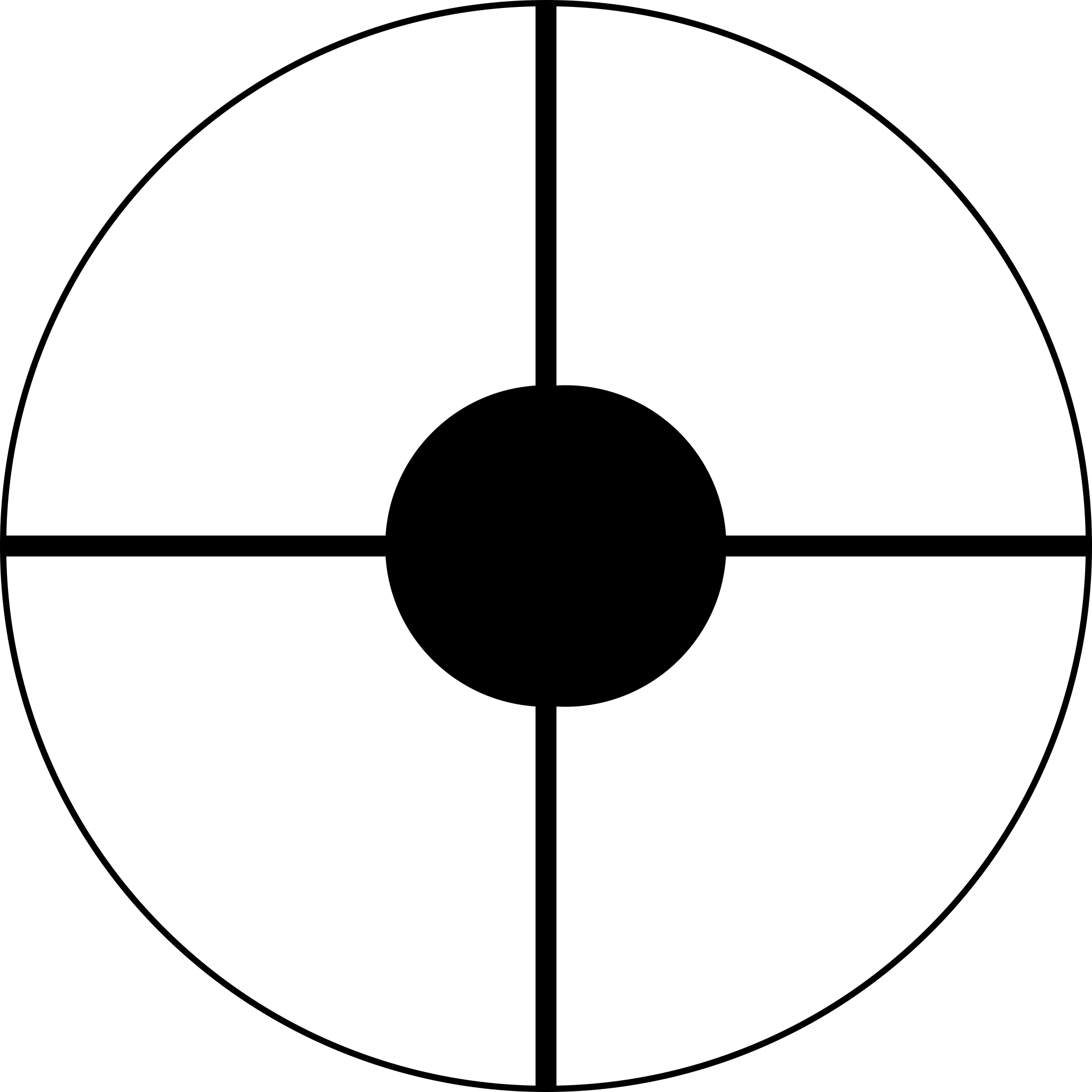
This PNG image must be placed in the same directory as the model with a representative name (e.g. obstruction.png), and referenced from the model inside an Obstruction element. We are going to place this element exactly where the M2 is located. The final model looks like this:
parameter focalLength = 1200e-3; # Focal length of the telescope [m]
parameter M2Position  = 900e-3;  # Location of the secondary mirror [m]
parameter M1Diam      = 254e-3;  # Diameter of the primary mirror [m]
parameter CCDRows     = 1024;    # Vertical resolution of the CCD
parameter CCDCols     = 1024;    # Horizontal resolution of the CCD
parameter CCDPixSize  = 15e-6;   # Side of a pixel [m]

parameter M2Width     = 7.7e-2;  # Width of the secondary mirror [m]
parameter M2Height    = 11e-2;   # Height of the secondary mirror [m]
parameter M2YOffset   = 4.68e-3; # Vertical offset of the secondary mirror [m]
parameter AperturePos = 1000e-3; # Position of the aperture stop
parameter ApDiameter  = 260e-3;  # Diameter of the aperture

ParabolicMirror M1(focalLength = focalLength, diameter = M1Diam);

on aperture of M1
  translate(dz = AperturePos)
    ApertureStop telescopeStop(diameter = ApDiameter);

on vertex of M1 {
  translate(dz = M2Position) {
    Obstruction M2Support(diameter = 260e-3, file = "obstruction.png");

    rotate(180, 1, 0, 0) rotate(45, 1, 0, 0) {
      translate(dy = M2YOffset)
        FlatMirror M2(width = M2Width, height = M2Height, vertexRelative = true);

      rotate(45, 1, 0, 0)
        translate(dz = focalLength - M2Position)
          Detector det(
            rows = CCDRows,
            cols = CCDCols,
            pixelWidth  = CCDPixSize,
            pixelHeight = CCDPixSize);
    }
  }
}

path telescopeStop to M2Support to M1 to M2 to det;
If we repeat the simulation, we will see that the obstruction casted a shadow on the elements, starting from M1: